ABSTRACT
This document deals with artificial neural networks, starting from a generic introduction on their structure and main use, and going through a detailed explanation that clarifies the most characteristic aspects. Then are discussed the different types of networks, the different training methods, their most common applications, advantages and disadvantages.
INTRODUCTION
An artificial neural network is a computational model for representing a network of interconnected artificial neurons. The models, which consist of graphs with interconnected nodes (that are transcendent mathematical functions) by arches, clearly have a lower degree of complexity than biological neural networks, but, nevertheless, they represent excellent solutions for the now established artificial intelligence systems.
The ways to create an artificial neural network are both software and hardware, and the fields of application are innumerable(especially in control systems).
Development began in the 1950s and 60s although very slowly, the limits of the networks didn’t allow for a fast evolution. Subsequently, in the 80s, this had a revival thanks especially to the works of Hopfield and Rumelhart.
The first one focused on the use of networks with feedback mechanisms (graphs with loops), the second one, instead, on backpropagation training and feedforward (acyclic graphs). These networks could learn through a set of input – output examples.
The training algorithm makes it possible to bring the answers provided by the network closer to the desired answers from the training set by adjusting the weights associated with the arches of the graph.
This ability to learn from the data provided with the training set allowed at first to better understand the biological mechanisms of neural connections, but above all it gave results in a wide range of applications never achieved before.1
DETAILED EXPLANATION
As mentioned in the introduction, a network of artificial neurons can be represented by a graph whose elements (nodes) are interconnected by means of arcs.
Each node (or neuron) of the graph mathematically represents a transfer function (typically non-linear). If we consider the transfer function form, it is like
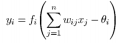
Where:
- •yi : output of node y;
- xj : input of node j;
- wij : weight of the arc between the node i and the node j;
- θi : is the threshold (or bias) of node i for the returned output.
A transfer function thus defined is of the 1st order.
The order of a node is defined as the number of inputs it receives, if we consider a node of the second order its transfer function changes to:
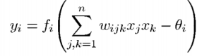
then the weight of the arcs between nodes i, j and k, the input from node k and node j are reported. Yi represents the output of node i of the second order.
The architecture of the ANN is determined by its topology, by the total connectivity and by the transfer functions that characterize each node of the network.2
Artificial neural networks must finally be regulated and the learning algorithms are precisely inspired by the dynamic architecture of biological neural networks in the brain. This can be very complex, if we consider biological networks the inputs and outputs of each neuron change as a function of time in the form of spike pulse trains.
A further degree of complexity is given by the architecture itself which is not static, but rather varies over time: learning, in fact, generates new neural connections (the arcs of the ANN graph and the axons of the brain).
Learning algorithms for ANNs refer to ideal neuronal models, but are based on the same fundamental principle that learning involves the regulation of neural connections. Therefore, the more finely the ANN is regulated, the greater the efficiency in data processing.3
The essence of a learning algorithm is therefore the modification of the weights associated with the arcs (neural connections), this modification is dictated by the learning rule: very common examples are the delta rule, the Hebbian rule, the antiHebbian rule, and the competitive learning rule.
Furthermore, the learning of the ANNs can be divided into 3 different methodologies:
- Supervised learning → It is based on the comparison between the output returned by the ANN network for a given input and the desired output. The algorithm in this case must minimize an error function such as, for example, the total mean square error between the output obtained and the desired output summed over all available data. An algorithm that applies this methodology is the backpropagation (BP) which is used iteratively to minimize the error;
- Reinforced learning → It represents a particular case of supervised learning. In this case the only information available is whether the output returned is correct or not, the desired output is “hidden”;
- Unsupervised learning→ in the absence of supervision, this method is based exclusively on the correlation between the data inputs. In fact, no information is available on the correctness or otherwise of the output.2
Unsupervised learning is currently not well understood. In this case it is the network itself that decides with which functionality to group the input data, this is defined as adaptation to the environment. There continues to be research in this field especially with regard to robots, these, in fact, could learn on their own when they encounter new situations or new environments for which there is no specific training set. The main difference therefore is that these networks do not use external influences to regulate the weights of the connection arcs, but rather self-monitor their internal performance.
The learning rules guide the action of the learning algorithms. Many of these laws are the variation of the oldest and most known rule, the Hebb rule.
Among the main learning laws we distinguish:
- Hebb’s rule: if a neuron receives an input from another neuron and they are both highly active (i.e. if mathematically they have the same sign) the weight of the neural connection between the two must be strengthened;
- Hopfield’s Law: it is inspired by Hebb’s law, but specifies the extent of the strengthening or weakening of the neural connection (weight).
It states, “if the desired output and the input are both active or both inactive, increment the connection weight by the learning rate, otherwise decrement the weight bythe learning rate.”; - The Delta rule: it represents a further variation of Hebb’s rule, it consists in continuously modifying the strength of the neural connections to minimize the mean square error between the output obtained and the desired output. When using this rule you have to make sure that the input data set is well randomized so that the network is finely tuned.
The rule is to transform the delta error in the output layer by the derivative of the transfer function and is then used in the previous neural layer to adjust input connection weights; - The Gradient Descent Rule: this rule uses the same method as the delta rule, but here, however, there is also an additional proportional constant related to the learning speed which affects the final modify factor acting on the weight;
- Kohonen’s Learning Law: this rule is inspired by the learning of biological neural systems. With this rule, the processing elements compete with each other in order to update their weight.
The element that returns the highest output is declared the winner and can inhibit its neighboring processing elements as well as excite them. Only the winner and it’s neighbors can change their connection weights. 4
TYPES OF NEURAL NETWORKS
Depending on the learning rule and the network architecture, we distinguish different types of ANNs. Some problems require the use of a specific type of ANN, while others can be solved with different types.
Among these ANNs we find:
- Hopfield networks: It is used efficiently for optimization problems. It can only be applied to binary inputs and implements an energy function;
- Adaptive resonance theory (ART) networks: ART networks are trained unsupervised. They therefore adapt to the information environment. They can be used effectively for optimization problems (such as Hopfield networks).
- Kohonen networks: They are trained unsupervised but the context of optimal application changes. They are in fact widely used to compress large data into smaller data while preserving their content;
- Backpropagation networks: They are networks widely used for data optimization (modeling, classification and control) and for image compression. The term backpropagation refers to the way the error returned at the output level is propagated backward to the hidden layer, and finally to the input layer;
- Recurrent networks: In recurrent networks, outputs from neurons are returned to the same neurons or to other neurons in different layers. The flow then follows different directions. Due to this particular architecture it is necessary to use specific training algorithms;
- Counterpropagation networks: These networks are trained through hybrid training to make a self-organized lookup table useful for function approximation and classification;
- Radial basis function (RBF) networks: These are a special case of feedforward error propagation network with three-layer.5
APPLICATIONS
Neural networks are a great way to manage and solve problems that cannot be characterized by a simple and specific representation. The fields of application are innumerable, for example they are used for control systems, in robotics, in pattern recognition, for prediction, in the medical field, in optimization and signal processing up, and also in the social / psychological sciences.6
In the case of prediction, the ANN networks can be used to predict the use and energy savings achievable with the renovation of buildings and their systems (for example refrigeration). In this field they would be very useful for building engineers by providing a general model which with such slight modification can also be used for other buildings.7
ADVANTAGES / DISVANTAGES
Using ANN has several advantages and disadvantages. Among the advantages offered, the main ones are:
- Storing information on the entire network: the loss of some information in some points of the network does not imply its malfunction;
- Ability to work with incomplete information: Since the networks are trained they are also capable of providing an output with missing pieces of input information. However, the performance degradation will be determined by the importance of the lost information;
- Gradual corruption: The network can deteriorate and slow down in response over time but this doesn’t imply its immediate malfunction;
- Machine learning: These networks make decisions considering events similar to those in input;
- Parallel processing capability: Due to their architecture they can perform more than one task at the same time.
And the main disadvantages are:
- Hardware dependence: due to their structure they necessarily require processors with parallel processing power. The realization of the architecture is dependent.;
- Unexplained behavior of the network: This is the most important problem of ANN. When ANN produces a probing solution, it does not explain why and how;
- Determination of ideal network structure: this is often done by trial and error because isn’t available an exact and specific rule to determine the ideal structure of artificial neural networks;
- Difficulty of showing the problem to the network: before being introduced into the network, the problems must be characterized and translated into numerical values so that the network can work on them.8
CONCLUSION
As previously described, artificial neural networks have several advantages that give them the role of a powerful computational tool for solving scientific and engineering problems. At present, however, they have limitations in replacing traditional methods such as statistical regression, or pattern recognition. Certainly over time, and through research, they will be able to improve and become more useful in other areas. The fusion of traditional methods and ANNs could be the real turning point.9
In fact, the computing world has a lot to gain from neural networks. Their main advantage of self-learning through examples makes it possible to use them in different applications without the need to write a specific algorithm to perform a single task. The research for further applications continues with confidence for the future.10
LIST OF REFERENCE
1. Terrence L Fine (1996) ‘Fundamentals of Artificial Neural Networks – Book review’ [Online], available at:
2. XIN YAO (1999) ‘Evolving Artificial Neural Networks’ [Online], available at:
3. BERNHARD MEHLIG (2021) ‘Machine learning with neural networks. An introduction for scientists and engineers’ [Online], available at:
https://arxiv.org/pdf/1901.05639.pdf
4. Dave Anderson and George McNeill (1992) ‘ARTIFICIAL NEURAL NETWORKS TECHNOLOGY’ [Online], available at:
https://www.csiac.org/wp-content/uploads/2016/02/Artificial-Neural-Networks-Technology-SOAR.pdf
5. I.A. Basheer , M. Hajmeer ‘Artificial neural networks: fundamentals, computing, design, and Application’ (2000) [Online], available at:
6. Soteris A.Kalogirou (2000) ‘Applications of artificial neural-networks for energy systems’ [Online], available at:
https://www.sciencedirect.com/science/article/abs/pii/S0306261900000052
7. Melek Yalcintas, Sedat Akkurt (2005) ‘Artificial neural networks applications in building energy predictions and a case study for tropical climates’ [Online], available at:
https://onlinelibrary.wiley.com/doi/abs/10.1002/er.1105
8. Maad M. Mijwil (2018) ‘Artificial Neural Networks Advantages and Disadvantages’ [Online], available at:
9. Yanbo Huang (2009) ‘Advances in Artificial Neural Networks – Methodological Development and Application’ [Online], available at:
10. Saumya Bajpai, Kreeti Jain, and Neeti Jain ‘Artificial
Neural Networks’ (2011) [Online], available at:
http://citeseerx.ist.psu.edu/viewdoc/download?doi=10.1.1.301.5738&rep=rep1&type=pdf