ABSTRACT
This paper deals with convolutional neural networks, starting from their introduction in terms of artificial neural network up to focusing on the most characteristic aspects of this particular type of neural network. After a mention on the history of their advent, the architecture of CNNs and the concept of convolution underlying these networks are discussed. The last part clarifies the main types of CNN networks, the differences in terms of applications, and their associated disadvantages and advantages.
INTRODUCTION
The CNN or ConvNet (convolutional neural network) is a particular type of Artificial Neural Network (ANN) specialized for the recognition of visual patterns, therefore images and videos. To fully understand how CNNs work, it’s necessary the knowledge of ANNs.
Artificial neural networks are computational systems inspired by the organization of biological nervous systems and their neurons. From the input layer to the output layer there are several layers of neurons (nodes) interconnected (through arcs) between them, they process the information according to a precise transfer function and contribute to the final output. The learning of such networks is typically carried out with a set of desired input-output examples through algorithms that allow to minimize the output error by modifying the weight of the neural connections (supervised learning).

Figure 1 – simple organization of an ANN
Another learning mode is the unsupervised, in this one the network doesn’t know the desired output but self-learns by monitoring its own internal processing environment.
Typically the best and most used learning for networks dedicated to image recognition is the supervised.1
One of the best known neural networks is CNN (convolutional neural network). This network takes its name from the mathematical operation of convolution(operation that can be applied to matrices) where convolution consists in integrating the product between a first function and a second transferred function of a certain value.
The convolution operation is therefore related to the correlations between matrices, where the matrices represent the images to be recognized by the neural network. The CNN, according to the ANN structure, includes different layers such as convolutional layer, non-linearity layer, pooling layer and fully connected layer.
The first two layers, the convolutional and nonlinear, are parameterized.
The other two layers, the pooling and fully connected, haven’t particular parameters.
CNNs are excellent and particularly suitable for applications involving image data such as largest image classification data set (Image Net).
Image Net, in fact, is a large database of images, created for use, in the field of artificial vision, in the field of object recognition.2
HISTORY
The history of CNN is closely related to the history of the ANN networks. In the last few years in particular, a great interest in deep learning has emerged and CNN networks have become the most established algorithm among the various deep learning models.
Such networks have established themselves as the dominant method in computer vision since the results obtained from their use have been shared in the object recognition competition known as the ImageNet Large Scale Visual Recognition Competition (ILSVRC) in 2012. Interest has further increased thanks also to the results obtained in the medical field.
Gulshan et al. , Esteva et al. , Ehteshami Bejnordi et al. , have demonstrated deep learning potential for diabetic retinopathy screening, skin lesion classification, and lymph node metastasis recognition, respectively.
Since then, several studies have been conducted and published. This advanced methodology, in fact, would help not only researchers using CNNs in their radiology and medical imaging tasks, but also clinical radiologists (as deep learning may influence their practice in the near future).3
DETAILED EXPLANATION (DESCRIPTION)
CNNs are a particular model of ANN composed of neurons (nodes) interconnected and distributed in different layers. An important feature of CNNs, which differentiates them from ANNs, is the ability to obtain abstract information from the input as it progresses into the deeper layers of the network. This feature makes them particularly suitable for image recognition: in a first level, in fact, the edges of the image would be recognized, while in the following the shapes that gradually take on more and more details.
So let’s suppose that the neural network receives an input color image of size 32×32 and depth 3 as RGB channel. We also suppose that this image is read in input as a set of raw pixels. So if we were to connect the input to a single neuron present in a subsequent hidden layer of the network, a connection with a weight of 32x32x3 would be required. Similarly, if we were to add another neuron in the same layer, an additional connection with weight 32 × 32 × 3 would be required, which will become in total, 32 × 32 × 3 × 2 parameters.
Clearly a network described in this way is not suitable for the complete classification of an image, which requires particularly complex networks in terms of topology and architecture, but we could think of using it to recognize the edges of the input image. However, this network (fully connected) needs 32×32×3 by 32×32 weight connections, which are 3,145,728.
Convolution is a more efficient method which consists in detecting different regions of the same photo as inputs: in this way the neurons hidden in the next level receive only inputs
from their corresponding part of the previous level, as shown in the next image.

With this mode, an alternative to the fully connected network, less intricate and more efficient networks are obtained. For example, it can only be connected to 5 × 5 neurons. So if we want to have 32 × 32 neurons in the next layer, we will have 5 × 5 × 3 connections for 32×32, or 76,800 connections (compared to the previous 3,145,728).
Another hypothesis to simplify it further is to use the same local connection weights to connect the neurons of one layer to all the neurons of the next layer. In this way the neighboring neurons of the next layer are connected with the same weight to the local region of the previous layer. Therefore, it again reduces the number of weights to only 5×5×3 =75 to connect 32×32×3 neurons to 32×32 in the next layer.
These assumptions, however approximate, allow to obtain advantages such as the reduction of the number of connections, but above all the possibility to slide internal windows (portions) of the image, by fixing the weights for the local connections, to the input neurons and mapping the output in the corresponding position.
It provides an opportunity to detect and recognize features regardless of their positions in the image. For this reason they are called convolutional.
To make the method even more efficient, it is possible to add further layers after the input level which are composed of neurons that look at the same portions of the image, but which extract different information and thus behave as image filters.
In the convolutional neural network these filters are initialized and followed by the training procedure shape filters.2
The focal point of the CNN networks, from which they also take their name, is the convolutional layer. Convolution is a mathematical operation between an input I and an argument, the kernel K, which returns the cross-correlation between the two. In other words, it expresses how the shape of one is modified by another.
CNNs handle image data, so the convolution in terms of images is explained below.
The input image is called “x” and represents a 2D array with different color channels (red, green and blue-RGB). The feature detector, or kernel, “w” is applied to the input according to the convolution product, so we get the feature map. The convolution function applied is:
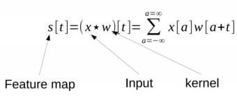
The convolution operation allows to calculate the similarity between two signals, so we could use a feature detector as a filter to identify, for example, the edges of the image. The basic assumption in CNNs is that the convolution function is initialized to 0 everywhere except in the finite set of points for which we store values. The infinite summation therefore results in a finite summation on a certain number of elements of the array.


As mentioned in the introduction, there are additional fundamental layers in CNNs. The next is the non-linearity layer. This can be used to adjust or cut-off the generated output.
Its use is therefore necessary to saturate the output or limit the output generated. For many years, sigmoid and tanh were the most popular non-linearity. The last two levels, instead, are the pooling and the fully connected layer.
The function performed by pooling is down-sampling in order to reduce complexity for further levels (without affecting the number of filters). The operation performed can be considered similar to reducing the resolution and one of the most applied methods is Max-pooling.
In this case, the image is partitioned into sub-regions and the method returns the maximum value of each sub-region. One of the most common sizes used in max-pooling is 2×2.
Finally, the fully connected layer resumes the organization of traditional neural networks. In fact, in this layer each node is connected to each other node of both the previous and the next layer. The disadvantage introduced by the fully connected layer are obviously the numerous parameters that require a complex calculation in training examples.
The essence of a CNN network is therefore the organization and the number of different types of layers chosen for its implementation, so these characteristics allow to identify different types of CNN.2
TYPES OF CNN
An event is held annually called the ImageNet Large Scale Visual Recognition Challenge (ILSVRC) which consists of large-scale object detection and image classification using CNN. Different types of CNNs that represented a point of reference in the field of object classification. will be discussed below.
LeNet , initially conceived and trained to classify the handwritten digits 0 to 9 of the MNIST dataset, was one of the most revolutionary algorithms in its object classification capability.
Thanks its revolutionary nature, its layered composition will also be indicated below::
1. FIRST CONVOLUTIONAL LAYER: 6 filters of size 5 X 5, and a stride of 1;
2. AVERAGE-POOLING LAYER: size 2 X 2, and a stride of 2; 3. CONVOLUTIONAL LAYER: 16 filters of size 5 X 5, and stride of 1;
4. AVERAGE-POOLING LAYER: size 2 X 2, and stride of 2; 5. FIFTH LAYER: connects the fourth layer to a fully connected layer (composed by 120 nodes);
6. FULLY CONNECTED LAYER: composed by 84 nodes, deriving from the outputs of the 120 nodes of the fifth layer;
7. LAST LAYER: is the final classification layer that allows you to determine the output class of the last level. The classes are 10 relative to the 10 digits for which LeNet was mainly trained to classify.
The accuracy obtained is approximately 98.9%, this is guaranteed by the RELU activation function. This function can be applied effectively in recognizing handwritten digits, but it is not suitable for processing large images and for classification into more than 10 classes.5
AlexNext, designed by Alex Krizhevsky, Ilya Sutskever and Geoffery E. Hinton, won the ImageNet ILSVRC in 2012. In terms of architecture it is very similar to LeNet, but includes a much larger number of filters which allow it to classify among a large class of objects while maintaining high accuracy. Thanks to this architecture it can receive in input a color image (RGB) of size 224 X 224.
AlexNet was simultaneously trained on two Nvidia GeForce GTX 580 GPUs but more were needed as the high computational cost, dictated by the 62.3 million parameters of the network, requires billions of computing units.6
VGGNet 16, designed by Simonyan and Zisserman, finished second in the ILSVRC-2014. It was ale to achieve a top-5 error rate of 5.1%. Despite the large number of parameters the scheme that the network follows is quite simple, which is why developers prefer it in the field of feature extraction. The basic parameters, filter size and strides, are constant for both the pooling layer and the convolution layer.
The convolution layers has filters of size 3 X 3 and stride = 1. Max-Pooling layer has filters of size 2 X 2 and stride = 2. These types of layers are applied in a precise order throughout the network. The number of parameters is very high (140
million) and exceeds that of AlexNet, which explains the difficult implementation of the same network.7
GoogleNet was the winner of the 2014 ILSVRC CNN, hitting an error rate in the top 5 of 6.67% (very similar to human-level performance). Its absolutely incredible performance is due to a smarter implementation of the LeNet architecture. The basic idea is that rather than implementing convolutional layers with many parameters in different layers, it is more efficient to implement the convolution so that it converges into a result containing matrices from all the filter operations together (so we do all the convolution together). The idea is called the initial module, from which the network is also named. This, in fact, can be called both GoogleNet and Inception Network.8
APPLICATIONS
The number of applications in which CNNs are involved has grown over time thanks to the evolution of this technology. Some of the most popular are mentioned below:
1. Image Classification: In the classification of images, the CNNs have made several steps forward. Their classification capacity and high accuracy has particularly evolved over time, in particular since AlexNet’s victory in ILSVRC 2012. From then on, the researchers made significant improvements in terms of filter size (reduction) and network depth;
2. Object Detection: Object detection is a long-standing data problem in the field of computer vision due to the difficulties that have arisen in how to precisely and accurately locate objects in images or video frames.
The idea of using CNNs in this area dates back to the 1990s, but development was nevertheless limited by the technologies of the time. After the excellent results of the CNNs in 2012, interest was reborn and the evolution continued with remarkable speed compared to the past;
3. Object Tracking: The main challenge is the representation of the target with respect to variables such as point of view changes, lighting changes and occlusions. With the necessary architecture changes it was possible to change the nature of CNNs from detector to locator;
4. Pose Estimation: DeepPose was CNN’s first application to the human pose estimation problem. In this work, the estimate of the pose is formulated as a regression problem based on CNN at the coordinates of the joints of the body. 7 layers in cascade were needed to think about the pose in a holistic way;
5. Text Detection and Recognition: OCR (optical character recognition) has always been one of the areas of greatest application of CNNs. It was initially developed to recognize characters on fairly regular images (well-aligned text and clean background), but recently the focus has shifted to text recognition on scene images due to the growing trend of high-level visual understanding in computer vision research;
6. Visual Saliency Detection: This technique, visual saliency prediction, consists of detecting important regions in images. As this is a very complex challenge, a couple of works have recently been proposed to take advantage of the strong visual modeling CNN capabilities;
7. Action Recognition: Another very complex challenge is represented by the recognition of action, analysis of human behavior and classification of their activity based on the dynamics of movement. By breaking down the problem into two parts, such as analysis of the action in still images and in video, effective solutions have been applied that involve the use of CNNs9.
ADVANTAGES/DISADVANTAGES
The most evident advantages from the use of CNNs concern especially the high accuracy and precision in classification / prediction problems. Furthermore, the range of CNNs is quite varied, allowing them to be used in different applications. Previously, approaches to image processing and classification were based on hand-engineered capabilities, whose performance and accuracy drastically impacted overall results. Feature engineering (FE) is also a rather complex and expensive process, and cannot be generalized but must be repeated whenever the data set changes (i.e. when the specific application changes).
The mere fact of not requiring FE is a great advantage offered by CNNs, they ,in fact, can automatically identify the important characteristics during the training process. Generally they are also quite robust with respect to possible variations in lighting, background, size and orientation of the images.
The main drawback, however, is the time required for training and the need for large data sets.
Furthermore, the correct annotation of such data is a delicate process that should only be performed by domain experts. Finally, another drawback is the problems that could arise when using a pre-trained CNN on a similar but smaller data set.10
FUTURE INNOVATIONS
Since 1989 the improvements made to CNNs concern their architecture and can be distinguished in parameter optimization, structural regularization and reformulation. The most significant improvement obtained comes from the restructuring of the processing units and the design of new blocks, it is therefore reasonable to think that a further boost to their evolution in the future may start from this area. Further changes to their architecture could make CNNs more versatile and make them efficient and established even in very complex challenges such as object tracking and visual saliency detection.11
CONCLUSION
As seen convolutional neural networks differ greatly from other types of neural networks by presenting quite peculiar characteristics that make them generally more suitable for processing image data.
This paper has focused on their structure and current areas of application, but it is to be expected that, with further improvements and changes to the architecture of CNNs, they will grow even more in number in the near future.
LIST OF REFERENCE
- Keiron O’Shea, Ryan Nash (2015) ‘An Introduction to Convolutional Neural Networks’ [Online], available at:
https://arxiv.org/pdf/1511.08458.pdf - Saad Albawi, Tareq Abed Mohammed (2017) ‘Understanding of a Convolutional Neural Network’ [Online], available at:
https://www.researchgate.net/profile/SaadAlbawi/publication/319253577_Understanding_of_a_Convolutional_Neural_Network/links/5ad26025458515c60f 51dbf9/Understanding-of-a-Convolutional-Neural Network.pdf - Rikiya Yamashita, Mizuho Nishio, Richard Kinh Gian Do, Kaori Togashi (2018) ‘Convolutional neural networks: an overview and application in radiology’ [Online], available at:
https://link.springer.com/article/10.1007/s13244-018- 0639-9 - Renu Khandelwal (2018) ‘Convolutional Neural Network(CNN) Simplified’ [Online], available at:
https://medium.datadriveninvestor.com/convolutional neural-network-cnn-simplified-ecafd4ee52c5 - Yann LeCun, Léon Bottou, Yoshua Bengio, Patrick Haffner (1998) ‘Gradient-Based Learning Applied to Document Recognition’ [Online], available at:
http://yann.lecun.com/exdb/publis/pdf/lecun-01a.pdf - Alex Krizhevsky, Ilya Sutskever, Geoffrey E. Hinton (2012) ‘ImageNet Classification with Deep Convolutional Neural Networks’ [Online], available at:
https://papers.nips.cc/paper/2012/file/c399862d3b9d6b76c8436e924a68c45b-Paper.pdf - Karen Simonyan, Andrew Zisserman (2015) ‘VERY DEEP CONVOLUTIONAL NETWORKS FOR LARGE-SCALE IMAGE RECOGNITION’ [Online], available at:
https://arxiv.org/pdf/1409.1556 - Christian Szegedy, Wei Liu, Yangqing Jia, Pierre Sermanet, Scott Reed, Dragomir Anguelov, Dumitru Erhan, Vincent Vanhoucke, Andrew Rabinovich (2014) ‘Going deeper with convolutions’ [Online], available at:
https://arxiv.org/pdf/1409.4842.pdf - Jiuxiang Gua, Zhenhua Wangb, Jason Kuenb, Lianyang Mab, Amir Shahroudyb, Bing Shuaib, Ting Liub, Xingxing Wangb, Li Wangb, Gang Wangb, Jianfei Caic, Tsuhan Chenc (2017) ‘Recent Advances in Convolutional Neural Networks’ [Online], available at:
https://arxiv.org/pdf/1512.07108.pdf - Andreas Kamilaris, Francesc X. Prenafeta-Boldú (2018) ‘A literature survey on the Use of Convolutional Neural Networks in Agriculture’ Networks’ [Online], available at:
https://repositori.irta.cat/bitstream/handle/20.500.12327/815/Prenafeta_review_2018.pdf?sequence=2 - Asifullah Khan, Anabia Sohail, Umme Zahoora, Aqsa Saeed Qureshi (2020) ‘A Survey of the Recent Architectures of Deep Convolutional Neural Networks’ [Online], available at:
https://arxiv.org/ftp/arxiv/papers/1901/1901.06032.pdf